A bit of housekeeping! Since you care about tolerance analysis I'm guessing you also make 2d drawings. If so, you might be interested in how Five Flute can be used to streamline your drawing review process. Click here to see how it works, we'd love to help you if we can. Now on to the nerdy stuff! Cheers!

Introduction

The goal of this article is to familiarize you with how to conduct root sum squared (RSS) statistical tolerance analysis for mechanical engineering applications. The reality of designing physical products is that manufactured parts always have some degree of dimensional variance as a result of manufacturing processes. As engineers and designers, it’s our job to understand how this dimensional variance will impact the as-built functionality of the products we design. It sounds simple, but in practice it is a multidimensional challenge that requires a variety of mathematical and statistical tools to tackle effectively. In this article we’ll be building your foundational understanding of the RSS tolerance analysis method by first reviewing the underlying math and statistics, discussing the practical application to manufacturing problems, running through a few examples to put this knowledge into action, and then closing with key takeaways that you can apply to any tolerance analysis problem you face in your career.

Note: If you are interested in worst case and/or monte carlo analysis check out our ultimate guide to tolerance analysis.

The root sum squared (RSS) method - an overview

The root sum squared (or RSS) method is a statistical tolerance analysis method that allows you to simulate the expected outcome for a population of manufactured parts and their associated assemblies. But why is it even important to understand this method when specifying tolerances for production parts? Worst case tolerance analysis is almost always too conservative to apply to large manufacturing runs, resulting in an over specification of manufacturing tolerances (ie: tolerances are unnecessarily too tight). This results in extremely expensive parts and/or significant scrap as a result of rejected parts in quality control.

Simulating a population of manufactured parts

So how does RSS help us get past the shortcomings of worst case tolerance analysis for production runs? Fundamentally, RSS tolerance analysis leverages the fact that in an assembly composed of multiple parts, it is unlikely that all components will have as-manufactured dimensions that are both far away from the mean and all biased to one side of the target dimension (ie: all parts are too large). A much more likely outcome is that some parts will be larger than desired, and some parts will be smaller than desired. When these groups of parts are assembled, this symmetric variance results in a relatively low probability that the assembly will be out of tolerance despite sometimes large variances in individual dimensions.

RSS tolerance analysis is a method that allows you to characterize the variance in the manufacturing process of all critical dimensions, and then sum these individual dimensional variances to determine the behavior of a population of assemblies.

The normal distribution and it’s application in manufacturing

So how do you simulate the behavior of 1000+ mechanical assemblies? Statistical inference, that’s how! The key is to leverage the properties of the normal (or Gaussian) distribution. For many manufacturing processes, it is safe to assume that the critical dimensions of a part will follow a normal distribution with a mean and a standard deviation. The mean describes the average value (for a single dimension) of a population of parts, and the standard deviation describes the range of variability (again for a single dimension) across the entire population.

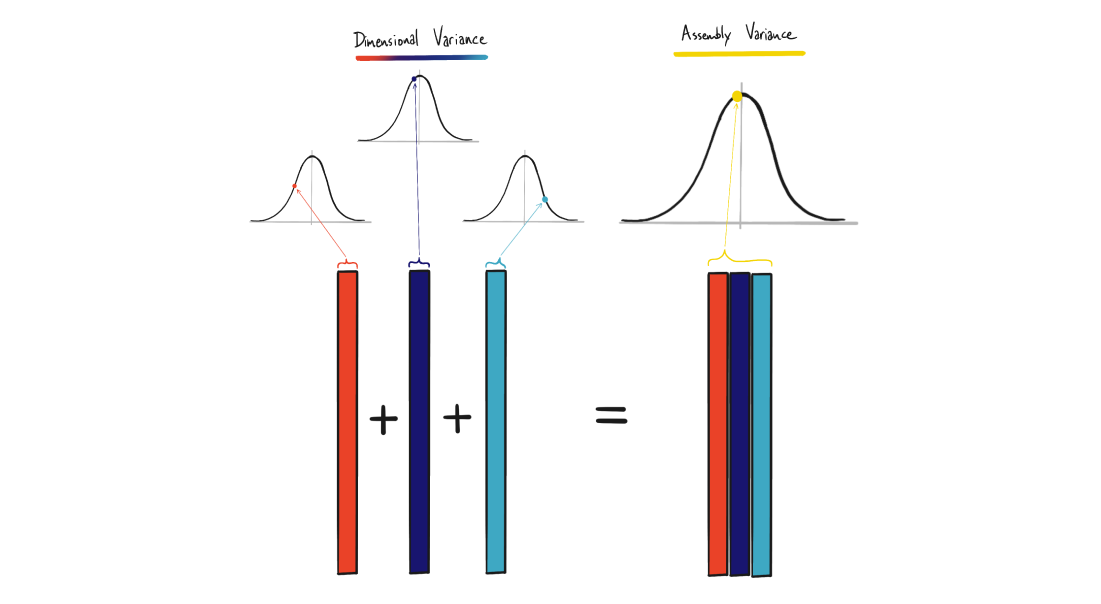
Take for example, the thickness of a cold rolled steel sheet. 14 gauge cold rolled steel sheet has a specified thickness of 0.075” and a tolerance of ±0.005”. Using a normal distribution we can safely assume that the average sheet thickness is 0.075”, meaning the manufacturing process is centered around the target specification. But how do we translate the specified tolerance into a dimensional variance that describes the range of thickness outcomes? A standard assumption is that a manufacturer will be able to produce parts such that three standard deviations fall within the specified tolerance range. In practice this means that 99.7% of all manufactured components will lie within the desired tolerance range

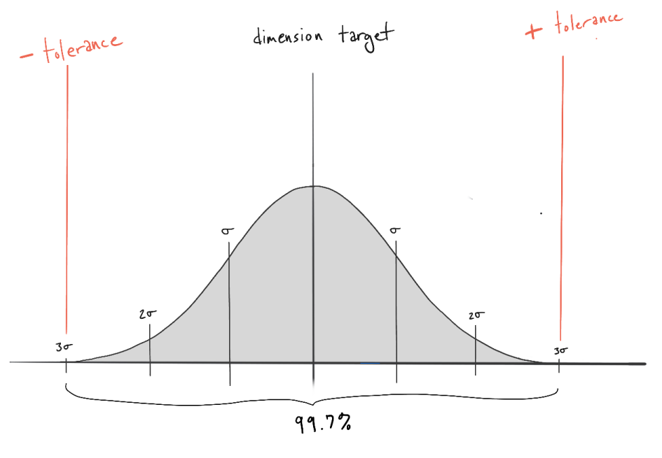
For our sheet metal example with a tolerance of ±0.005” the probability distribution looks like this. Note: the vertical lines represent standard deviations across the sheet thickness range.

So what exactly does this probability density function mean practically? You can think of it as a normalized representation of dimensional outcomes. A quick glance reveals that it is extremely unlikely that the sheet thickness will be below 0.0715” or above 0.0785”. Now imagine that two other manufacturers can supply 14 gauge sheet at thickness tolerances of ±0.002 and ±0.010 respectively. How likely will the average sheet purchased from each of these manufacturers fall between 0.0715” and 0.0785”? You can get a quick intuitive answer to this by plotting the probability density functions for all three tolerance values on the same plot. Note: the plot below includes standard deviations indicated by the vertical lines in colors corresponding to each tolerance specification.

Building your tolerance stack-up by adding variances and means

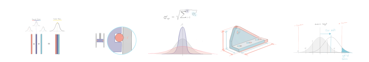
So what does this all mean in terms of assembly level behavior? For independent variables (like a critical dimension on multiple parts or different features of a single part) variances are additive. This incredible property allows us to sum variances across multiple dimensions and then compute a standard deviation for the entire system (or tolerance stack). By computing the system standard deviation and then applying that to the average value of the dimensional stack, you can build a probability density function for the functional assembly. This will allow you to simulate scrap or rejection rates for an entire manufacturing and assembly process with relatively straightforward math.

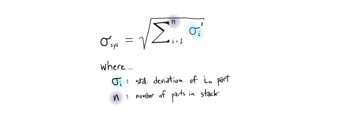
Here’s how you compute the system standard deviation.

Stacked sheet example

So let’s continue on with our sheet example but this time using three sheets stacked on top of each other. Let’s assume that the minimum allowable thickness of the three sheet stack is 0.216” and the maximum allowable thickness is 0.234” (ie: target stack thickness = 0.225 ±0.009”). Which of the three manufacturers can supply sheet that meets this assembly level target consistently?

Manufacturer A can produce 14 Ga sheet that is 0.075 ±0.002” thick at $25/square foot.

Manufacturer B can produce 14 Ga sheet that is 0.075 ±0.005” thick at $20/square foot.

Manufacturer C can produce 14 Ga sheet that is 0.075 ±0.010” thick at $15/square foot.

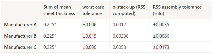
A back of the envelope worst case analysis would indicate that only manufacturer A can consistently hit a stack tolerance under ±0.009” but this may be unnecessarily costly. Applying the RSS method we can compute the system standard deviation for manufacturer B as follows.

Once you know the assembly standard deviation, you can compute the assembly symmetric tolerance by multiplying the standard deviation by three (remember our assumption about three standard deviations, or 99.7% of parts falling within the specified tolerance).

Results for all three manufacturers are shown in the table below.

Mean shifts and how to model process shift and drift

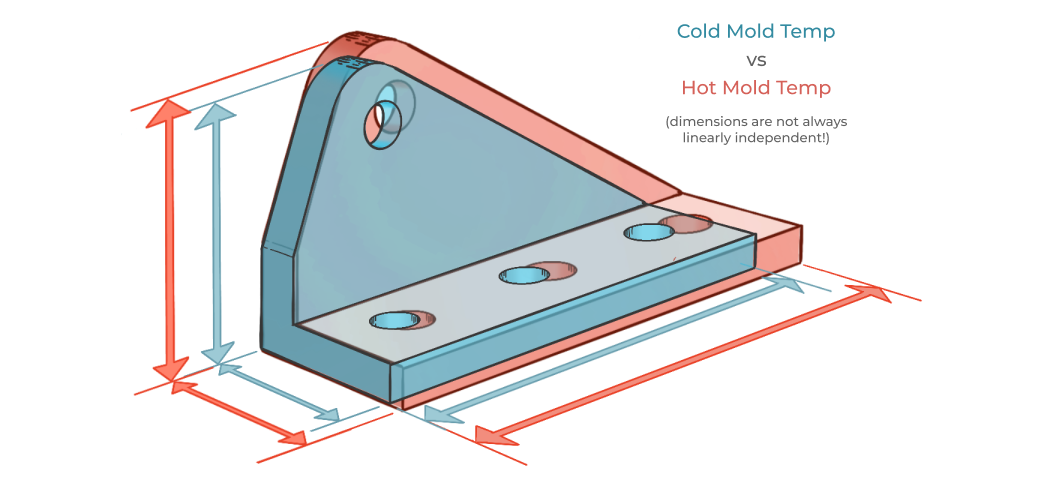
One of the key assumptions behind the RSS method is that dimensions are linearly independent (like orthogonal vectors). This is the reason that RSS tolerances are less conservative and more realistic than worst case tolerance analysis. In reality, however, not all dimensions of a part are guaranteed to be linearly independent. They may vary uniformly together, causing all critical dimensions to be larger or smaller than the specification.

Imagine an injection molding facility without indoor air temperature control. Despite individual mold cooling, the average temperature of the injection molding tool may be 50 degrees hotter during the summer months than the winter. This will result in significantly larger parts coming off the mold in the summer due to thermal expansion of the tool. This type of dimensional variance can be characterized by shifts in the mean value of the manufactured component’s critical dimensions.

A standard practice in RSS tolerance analysis is to analyze the impact of a mean shift of 1.5 standard deviations for one or more critical dimensions in the stack-up. Simply add (or subtract) 1.5σ to the mean (target specification) value of those dimensions that you think are subject to process drift or shift. Then compute your assembly tolerances as we did in the previous example.

Applying mean shifts to our 3 sheet example

Continuing on with our 14 Ga sheet steel example we can compute the impact of a 1.5σ mean shift on the assembly level performance. Remember that the mean shift does not impact the variance of the process. Recalculating the 3σ minimum and maximum material conditions for the stack-up while including a +1.5σ shift in mean thickness gives us the following results. Recall that the minimum allowable thickness of the three sheet stack is 0.216” and the maximum allowable thickness is 0.234” (ie: target stack thickness = 0.225 ±0.009”).

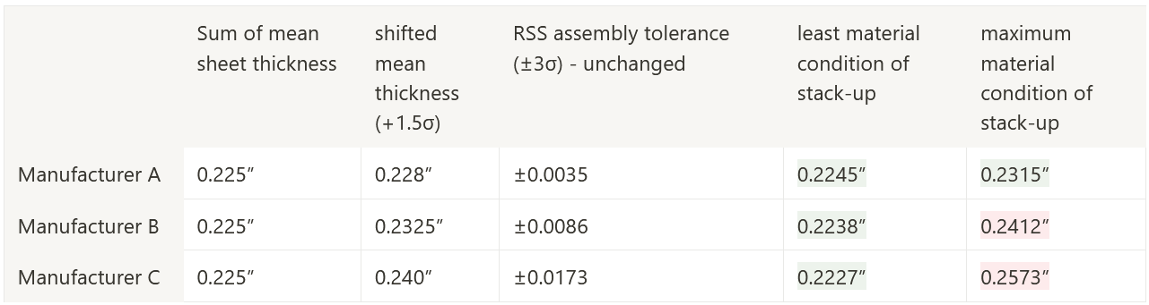
As you can see from the results, the mean shift is significant enough to cause the maximum material condition for the plates made by Manufacturer B to be out of spec. Note that this is no longer a symmetric failure as all assemblies fall within the least material condition limits. Mean shifts cause failures on either the left or right tail of the distribution.

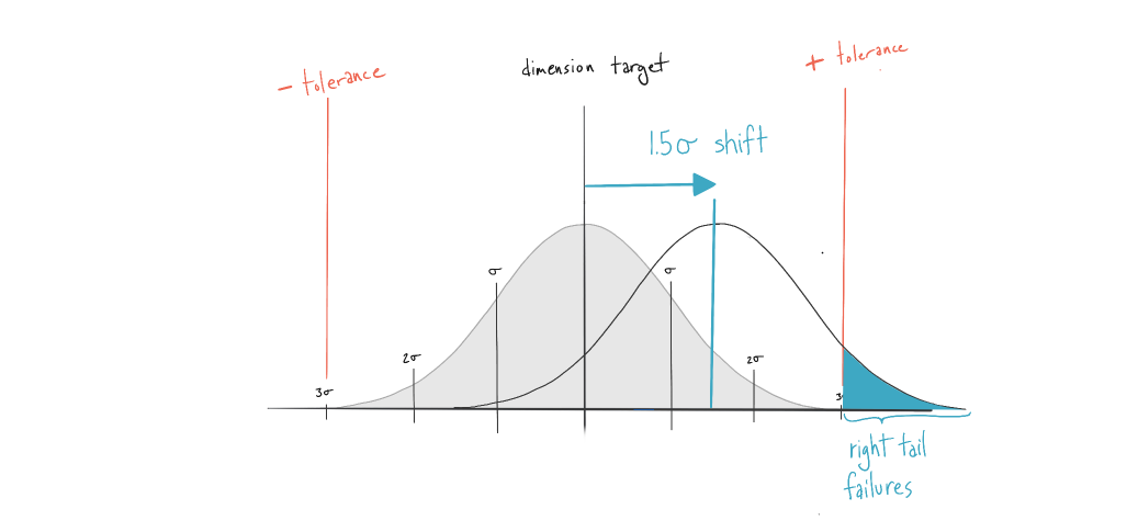
Returning to our thermal drift example for the injection molded parts, these asymmetric (tail biased) failures make sense intuitively when you think about how an increase in mold temperature would lead to larger parts, and assembly failures above the maximum material condition limit for the stack-up.

Piston o-ring example

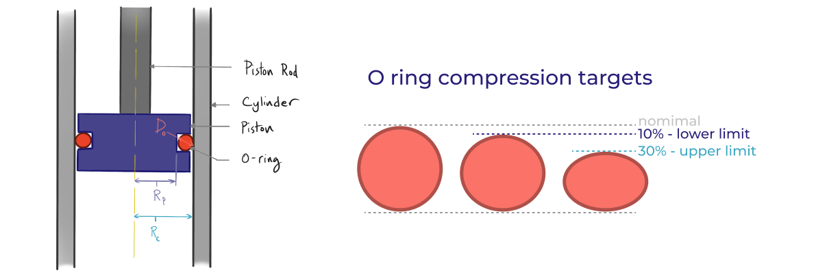
Now let’s put RSS into practice on a more realistic example. In this case you are designing a hydraulic piston assembly as part of a custom actuator project. The actuator body is comprised of an off the shelf cylinder, a custom piston rod, a machined piston, and an off the shelf 1/16 fractional, dash 032 o-ring seal. You have been given manufacturing tolerances for the cylinder inner diameter and the o-ring cross section diameter. You are designing a custom machined piston and you need to specify a machining tolerance for the inner diameter of the o-ring groove. The o-ring seal will function well if you maintain a static compression of 10% - 30% of the o-ring nominal diameter. The machine shop can hit a standard tolerance of ±0.005” on the piston diameter. Any further reduction in tolerance will increase machining cost. Will this standard tolerance work? If not, what is the tolerance that will ensure assembly functionality in production while minimizing machining cost?

Solution Steps

To solve this assembly tolerance problem we will go through the following steps.

1. Construct a tolerance stack equation to represent how the dimensions sum in the assembly.
2. Compute the acceptable limits for assembly behavior that satisfy the tolerance equation. You can think of this as establishing maximum and minimum material conditions, or go/no-go limits on the tolerance stack.
3. Calculate the standard deviation and variance for each dimension.
4. Plug the mean value of each dimension into your stack equation. Additionally, sum the variances of the individual dimensions and then take the square root of the sum of variances. This is your stack equation result and associated assembly standard deviation.
5. Convert from standard deviation back to a plus/minus tolerance at the assembly level.
6. Compare the assembly tolerance (via max and min conditions) to the limits established in step 2.
7. Iterate on individual component tolerances until you find a solution.

Solution

First build your tolerance stack equation to represent how the dimensions sum in the assembly. In this case we can construct a stack equation that sums the radial dimensions of the components and the diameter of the o-ring and computes the static o-ring compression, X.

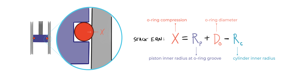
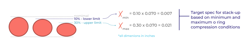
Then establish dimensional targets for the entire stack-up (ie: what conditions satisfy the tolerance equation). In our case, we first need to compute the target limits on o-ring compression in order for the seal to function (shown below as Xmin and Xmax).

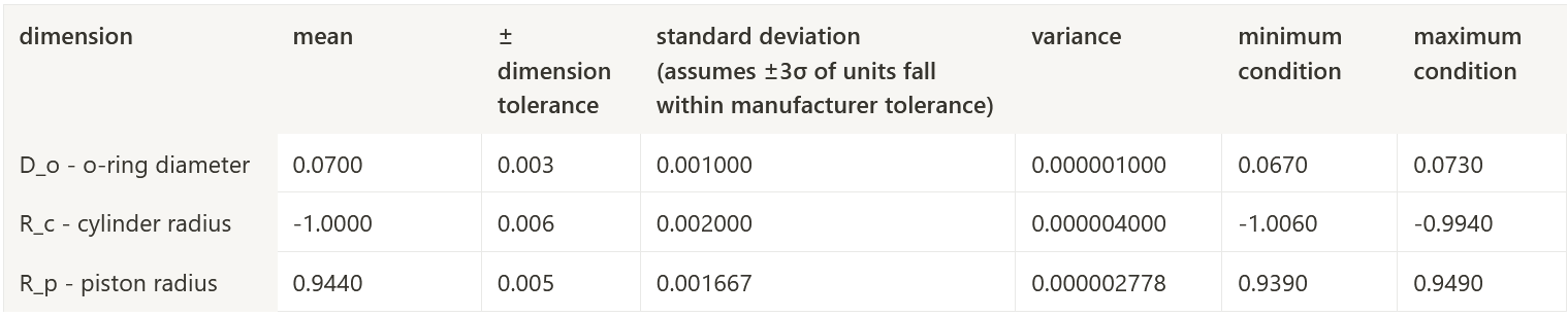
Now simply plug the mean value of each dimension into your stack equation to compute the nominal o-ring compression. Then calculate the standard deviation and variance for each dimension in the stack based on the tolerance for each dimension. Recall that we are assuming that the manufacturing process is capable of delivering 99.7%, or three standard deviations, of units within the specified tolerance. The variance is the square of this standard deviation. These values are shown in the table below, along with the minimum and maximum condition of each dimension.

Now you can compute the assembly standard deviation by summing the variances of the individual dimensions and then take the square root of the sum of variances. With the standard deviation in hand, you can convert back to a plus/minus tolerance at the assembly stack level by multiplying by 3 (unwinding our ±3σ assumption). Results for the assembly are shown below along with min and max conditions for o-ring compression based on the computed assembly tolerance.

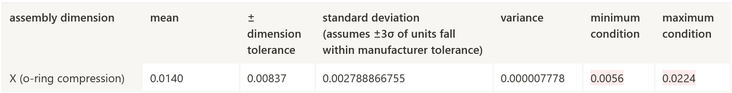
Now you can compare the minimum and maximum conditions for o-ring compression to the target specification for the stack-up that we computed in step 2. Recall Xmin (based on 10% compression) is 0.007”, which is above the calculated minimum condition of 0.0056” based on our RSS assembly tolerance. Xmax is 0.021”, which is below the calculated maximum condition of 0.0224” for the assembly. Based on these individual component tolerances, its safe to conclude the assembly tolerance is not sufficient to ensure that 99.7% of units will have a functional seal.

If however, we tighten the piston radius tolerance up from ±0.005” to ±0.0015” and recalculate the assembly tolerances...

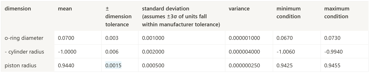
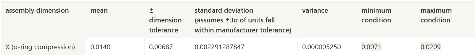
...you can see that the o-ring compression now falls just barely within the target spec! With RSS tolerance analysis it’s simple to iterate dimensional tolerances until assembly performance is within the target specification.

Takeaways

Key assumptions

In order to use RSS tolerance analysis in real world applications, it’s critical to understand the assumptions it is based on so you can apply it judiciously and accurately. The first assumption is that the manufacturing processes used to create all critical dimensions can be accurately modeled by the normal distribution obeying the central limit theorem. This implies that tolerances are symmetric around a mean target value. The second key assumption is that all dimensions are linearly independent, and to the extent that they do not behave this way, the behavior of the as-manufactured parts and as-built assemblies can be reasonably approximated by mean shifts representing process shift and drift due to external or endogenous factors. It’s your job as an engineer to think through these assumptions very carefully and apply the RSS method conservatively.

Pros of this approach

There are a few key advantages to the RSS tolerance analysis method that are worth highlighting.

• RSS tolerance analysis allows you to compute system level behavior for entire populations before you ever manufacture a single part. That alone is incredibly powerful!
• RSS tolerance analysis is generally much more realistic and less conservative than worst case analysis. This can reduce part cost by allowing you to relax individual dimensional tolerances to easily achievable levels while maintaining high quality at the assembly level. Your machinists and manufacturing partners will thank you!
• The RSS method is relatively quick and flexible and can be applied to most manufacturing processes. To the extent that a process doesn’t follow a perfect normal distribution or is likely to be impacted by external environmental factors, the mean shift computation offers a conservative method to understand how a manufacturing process will respond and perform under those external factors.
• The RSS method and careful application of confidence intervals allows you to estimate scrap rates in manufacturing. When a critical dimensions fall outside the desired specification, RSS and confidence intervals can allow you to compute the probability and estimated cost of those failures in production. This is invaluable when you encounter unexpected issues in production.

Cons of this approach

Conversely, there are a few disadvantages to the RSS tolerance analysis method that are important to understand before putting it into practice.

• The underlying assumptions that RSS is based on are not always true! It’s important to understand if the manufacturing processes involved behave in accordance with the above assumptions.
• Specifically, and perhaps most importantly, not all processes follow a normal distribution. Due to the fundamental physics of different manufacturing processes, the human error elements, internal and external factors, many processes follow asymmetric distributions where failures are expected to be biased towards one tail of the distribution. Instead of RSS, Monte Carlo tolerance analysis methods can be extremely helpful in these cases.

Closing thoughts

The RSS tolerance analysis method strikes the perfect balance of ease of computation, accuracy in real world applications, simplicity and extensibility to a variety of cases. Now that you understand the basics, give it a try on your project. Or check out our free online RSS tolerance analysis calculator. If you enjoyed this article or have any follow up questions please email support@fiveflute.com and we’d be happy to help.

Tolerance analysis and design reviews

Tolerance analysis is just one component of a good design review practice. If you struggle to get consistent and actionable feedback on your work, you should try Five Flute. It’s the fastest way to share, review, and improve your engineering designs.

Learn more: Here’s how Five Flute works for design reviews and drawing reviews.