(A bit of housekeeping! Since you care about tolerance analysis I’m guessing you also make 2d drawings. If so, you might be interested in how [Five Flute powers collaborative drawing reviews](/. Take a look, we’d love to help you if we can. Now on to the nerdy stuff! Cheers!)
Statistical tolerance analysis is a tool that every engineer should understand how to apply to their designs. Previously we covered the basics of statistical tolerance analysis in our introduction to root sum squared (RSS) tolerance analysis engineering guide. In this article, we’re going to explore statistical tolerance methods further to help you tackle (and recover from!) some of the trickier issues you are likely to face in production.
Background
In our introduction article we looked at a straightforward application of RSS tolerance analysis focusing on calculating assembly level behavior. This approach allows you to answer a simple question - what individual dimensional tolerances will result in an assembly tolerance that basically always works? It doesn’t however address what happens when things go wrong during manufacturing (as they often do).
The remainder of this article is going to focus on one key question: what happens when a manufacturer can’t hit the specified tolerance? We will unpack this question by looking at the application of statistical tolerance analysis to:
- Computing actual manufacturer performance
- projecting scrap rate % and costs
- Understanding and adapting to poor manufacturer performance
Quantifying Manufacturing Performance
The main assumption of RSS tolerance analysis is that the individual manufacturing processes can be modeled using a normal distribution. One of the first things you’ll want to check is if this normal distribution holds in the real world. In reality, you won’t know the mean and standard deviation for any particular dimension until a certain number of parts are made. But you can and should be computing dimensional performance early and often!
Passing the sniff test - does the data look normally distributed?
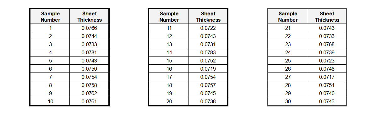
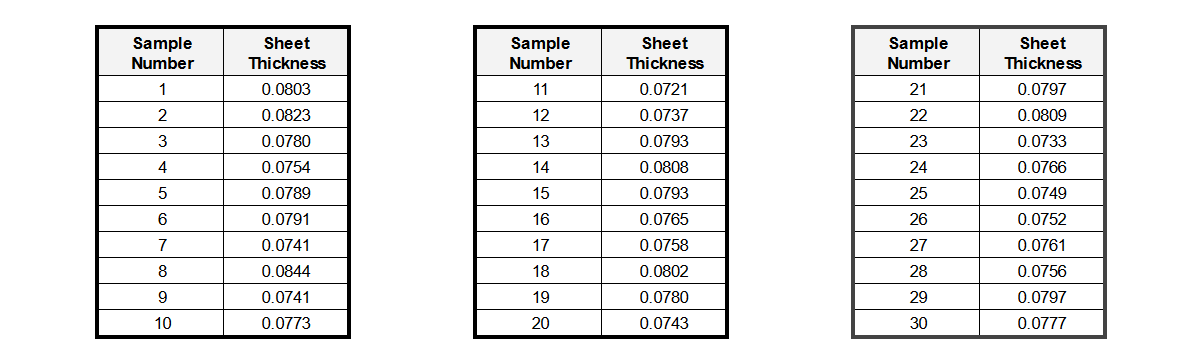
Returning to our example from the introduction to RSS article, let’s assume we are interested in the thickness of 14 gage (0.075”) mild steel sheet metal. The manufacturer promises a sheet thickness tolerance of ±0.005”. The first 30 production sheets you measure have the following thickness dimensions.
The first thing to do is plot the thickness data as a histogram and see how it looks.
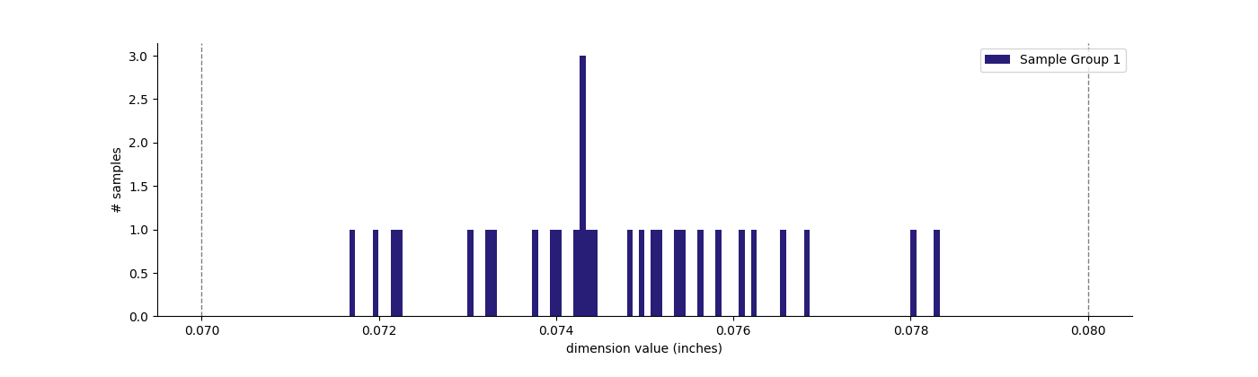
A histogram can give you a simple approximation of the shape of the probability distribution as well as confirmation that there are no significant outliers in the sample. Even with a relatively small sample size, the above histogram shows that the sampled data stays within the specified tolerance (marked by the vertical dashed lines) and appears roughly Gaussian (or normal) in shape.
Comparing expected to actual values for process mean and standard deviation
Setting aside sample size for the moment, the first step is to compute the mean thickness and standard deviation for the initial sample of 30 units. In this case we calculate a mean thickness of 0.07465” and a standard deviation of 0.00162”. We originally assumed that the manufacturer was capable of delivering plus or minus three standard deviations of units within our specified tolerance of ±0.005”.
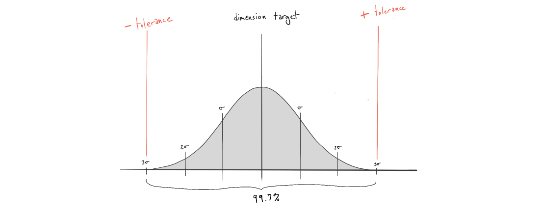
Dividing the symmetrical tolerance by three, we get a desired standard deviation of 0.00167” or less. Since our measured standard deviation (0.00162”) is less than the process expectation (0.00167”) we can expect that the manufacturer will most likely deliver sheets within our desired tolerance range moving forward (in the absence of any changes to the manufacturing process). You can confirm this visually by plotting the normal distribution of your expected vs observed performance.
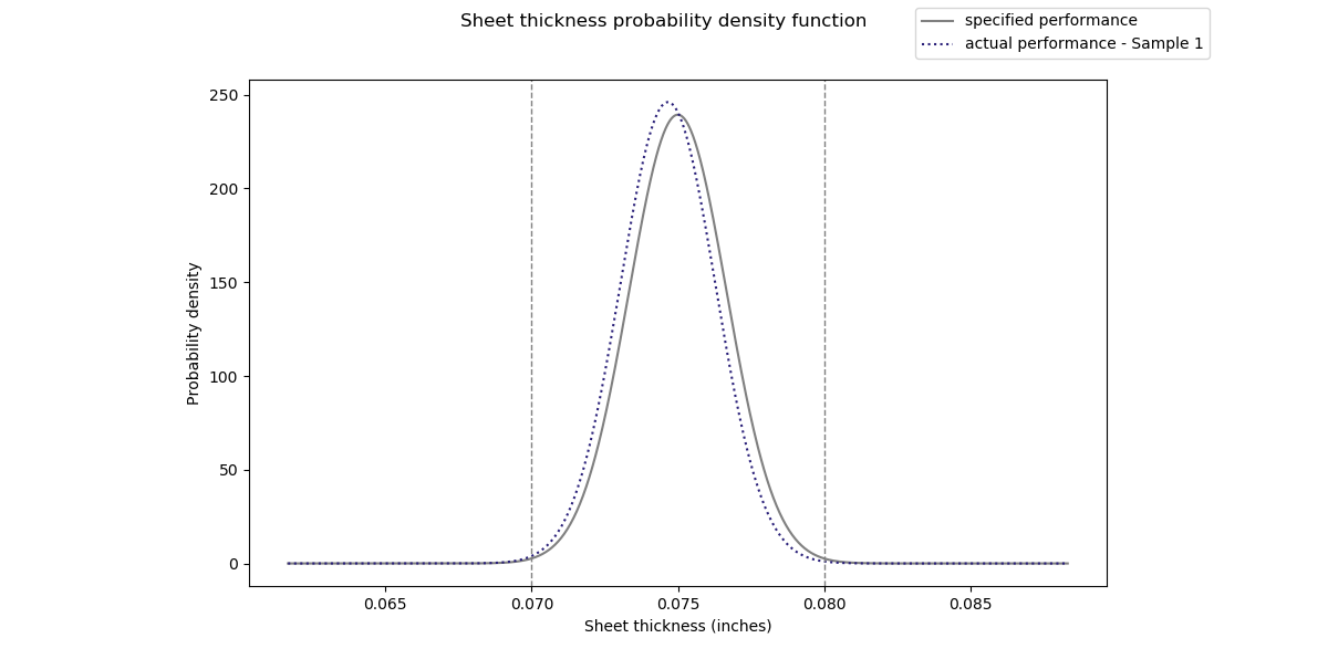
You can see from the two plots that, despite the small difference in mean and standard deviation, the vast majority of samples fall between the tolerance limits.
Assessing and Recovering From Poor Performance
But what happens if the manufacturer produces parts outside the desired tolerance range?
Lets analyze what to do in another scenario where the first 30 production sheets you measure have the following thickness dimensions.
As we did before, the first steps are to plot the samples as a histogram and compute the process mean and standard deviation. In this case we compute a mean thickness of 0.07746” and a standard deviation of 0.00288 (significantly greater than 0.00167”).
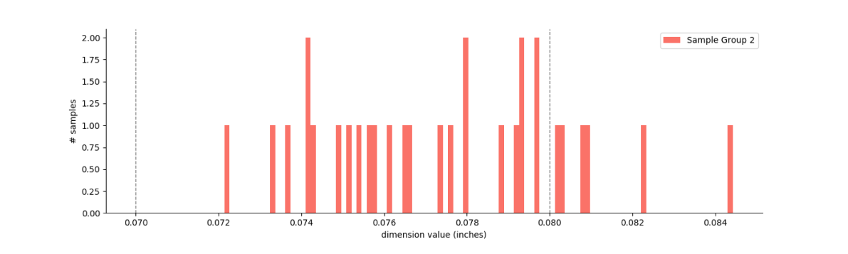
From the plot we can see that the distribution looks relatively normal, but it is not centered at our desired mean (0.07746” instead of 0.0747”) and there are several samples outside our desired tolerance range. But how costly will this be in real terms?
Calculating Scrap Rates and Failure Cost with Z-scores
We can tackle the cost problem by computing the number of failures and the cost of each failure. Based on our new understanding of the process, what percentage of units will fall outside our desired tolerance range? Let's start by plotting the normal distribution using our new process mean and standard deviation.
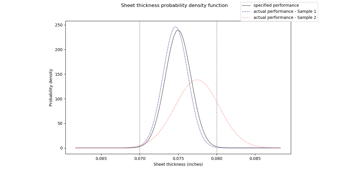
From the plot you can see that the vast majority of failures will occur on the right tail of the distribution. In our case this means that the sheet thickness of a large percentage of units will be oversized. But how many?
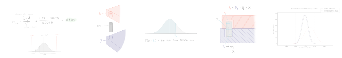
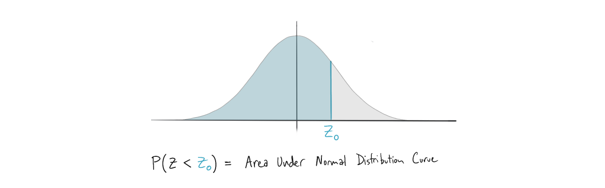
We can compute scrap rates (failure %) using z-scores and z-tables. Z-tables allow us to quickly compute the area under the probability density function for a given z value. The area under the distribution is equivalent to the probability of z being less than a specified upper limit (Zo), in our case the maximum sheet thickness.
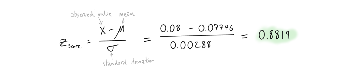
Start by computing the z-score of the tolerance limit (or observed value) relative to the mean of your sample population. In this case, the upper limit of sheet thickness is 0.08”. The z-score is a measure of how many standard deviations this limit is away from the mean sample population. We can calculate this as follows...
Then use a standard z-table to look up the probability associated with the above z-score.
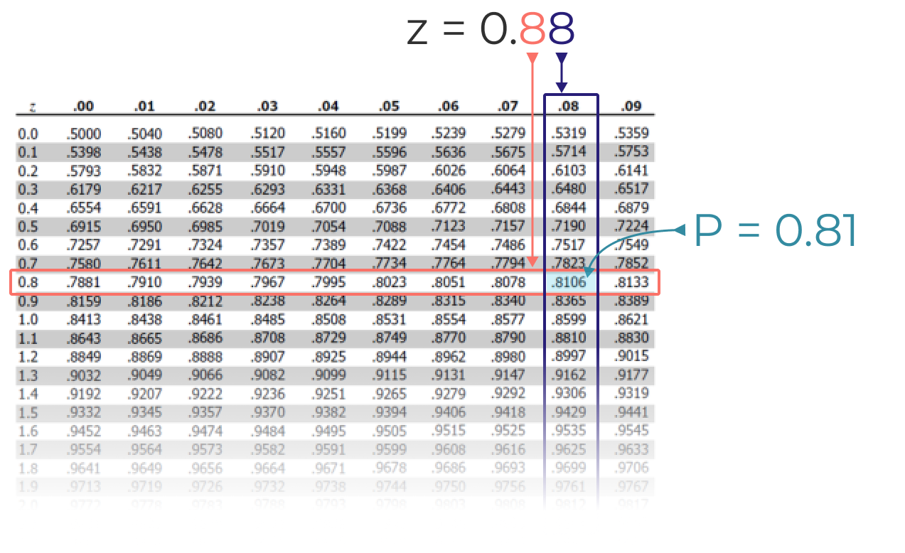
In this case we get a P value of 0.81, meaning 81% of all steel sheets will have a thickness below the upper tolerance limit of 0.80” and 19% of all sheets will be too thick.
You can use the same technique to compute how many sheets will be below the minimum thickness tolerance.
First computing the z-score...
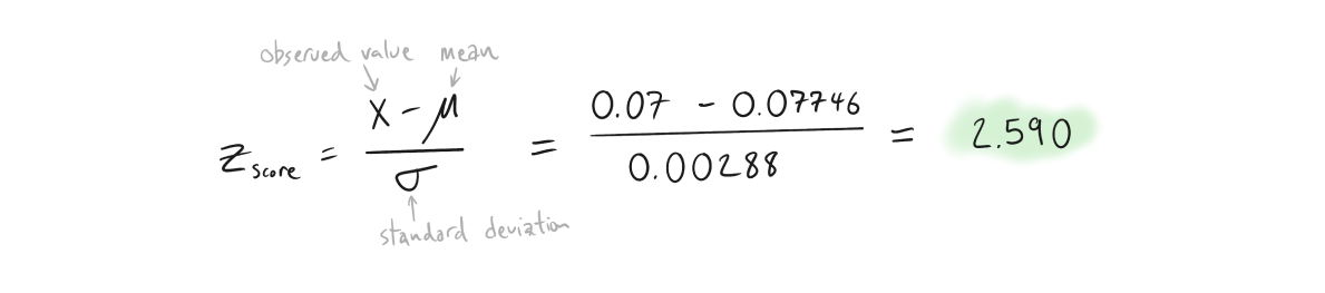
...and then using the negative z-table to calculate probability.
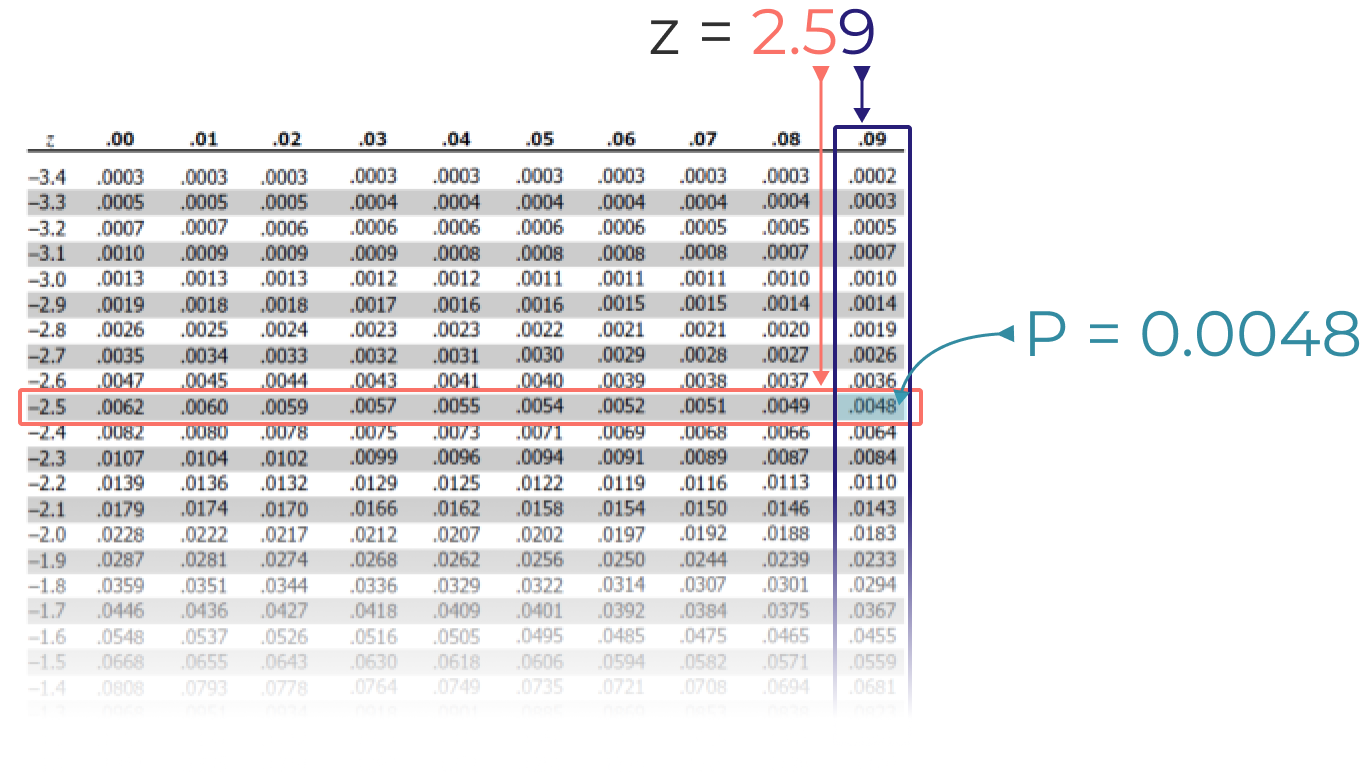
Since our P value is 0.0048, we estimate that approximately 0.5% of all units will have a thickness below the lower tolerance limit of 0.070”.
Combining left tail and right tail failures, we compute a total failure percentage of 19.5%. Computing cost is as simple as projecting the number of failures based on total production, and multiply by the unit cost of scrap. For example, if 20,000 units are produced you can expect 3900 steel sheets that fall outside the tolerance range (0.195 x 20,000 = 3900). If each sheet costs $2.00 you will have $7,800 of scrapped production units. It’s then up to you to determine if this is acceptable or not.
Assembly Example: Dowel Pin Alignment Stack-up
Suppose you are developing a product with critical alignment features controlled by a dowel pin. In this case, a 1/2” precision ground dowel pin is inserted into blind holes used to control the X-Y position of two machine components (we’ll call them A and B).
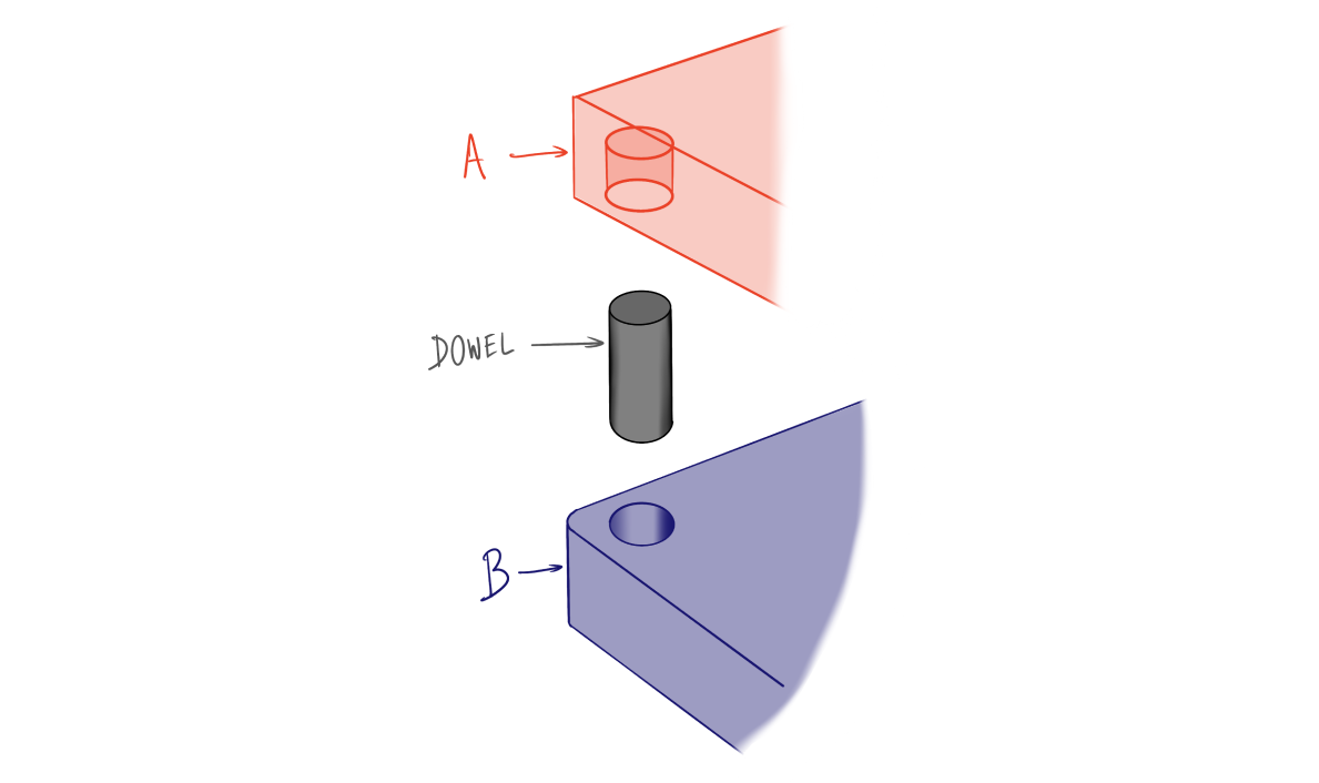
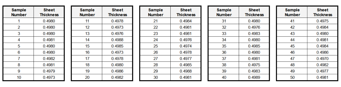
Component A has already been manufactured with a blind hole diameter of 0.502±0.0018” and samples confirm that the manufacturer is delivering on this specification with a process capability of 1.0, meaning 99.7% of all holes fall within the specified tolerance centered around the nominal hole diameter. After shipping to your assembly facility, the dowel supplier discovered an issue with their grinding equipment causing dowels to be undersized. Instead of holding an external diameter of 0.499±0.0008 they will now deliver dowels with a reduced diameter at an unknown tolerance. From an initial sample of 50 measured dowels, you record the following diameters.
Component B has a specified diameter tolerance of 0.502±0.0018” but has not yet been manufactured. For the assembly to function properly, a true position tolerance of 0.0025” must be maintained between component A and B at the dowel pin location. With the current manufacturer performance, what percentage of assemblies will be functional?
This is a complex scenario that we will answer by follow three major steps:
- Estimate the manufacturer performance for dowel pin diameter from our initial sample of 50.
- Build an RSS tolerance stackup for the entire assembly.
- Compute failure percentage using z-scores and z-tables.
Assembly Example - Estimating Dowel Pin Tolerance
As we did previously, start by plotting a histogram of the measured dowel pin diameters to determine if the manufacturing process can be characterized by a normal distribution.
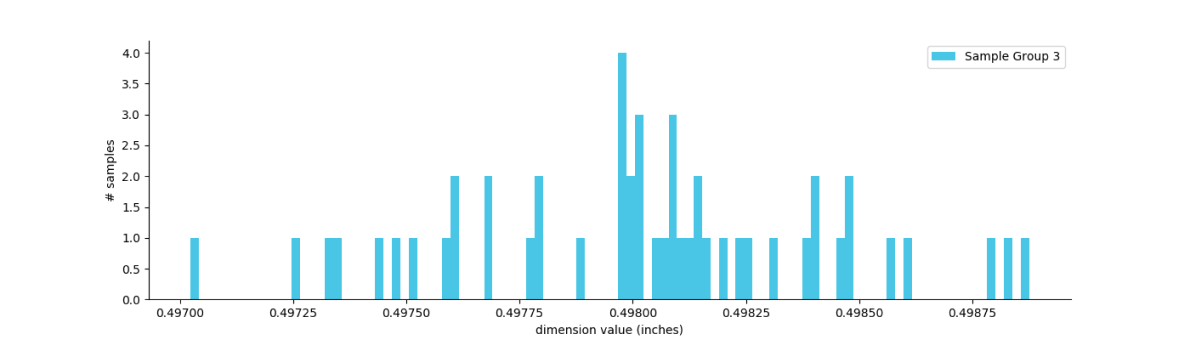
Then simply compute the mean and standard deviation for the sample set. In this case we calculate a mean diameter of 0.4980” with a standard deviation of 0.0004 and an associated tolerance of ±0.0012”.
Assembly Example - RSS Tolerance Stackup
Now build your RSS tolerance stackup for the entire assembly by following the steps from our introduction to root sum squared (RSS) tolerance analysis engineering guide shown below.
Basic solution steps for computing assembly level tolerances with RSS Method
-
Construct a tolerance stack equation to represent how the dimensions sum in the assembly. In this case we need to maintain a true position tolerance of 0.0025” between component A and B at the dowel pin location.
-
Compute the acceptable limits for assembly behavior that satisfy the tolerance equation. We know from our true position tolerance that X must be less than or equal to 0.0025”.
-
Calculate the standard deviation and variance for each dimension. (see table below)
-
Plug the mean value of each dimension into your stack equation. Additionally, sum the variances of the individual dimensions and then take the square root of the sum of variances. This is your stack equation result and associated assembly standard deviation. (see table below)
-
Convert from standard deviation back to a plus/minus tolerance at the assembly level. (see table below)
-
Compare the assembly tolerance (via max and min conditions) to the limits established in step 2. In this example, our computed maximum condition is 0.00375”, which is greater than our allowable deviation of 0.0025”. We know that there will be failures primarily on the right tail of the distribution in this case.
Now that the assembly level behavior has been characterized, you can compute the failure rate.
Assembly Example - Computing Failure %
Start by plotting the normal distribution of the assembly dimension (X) we are concerned with.
From the plot you can see that the vast majority of failures will occur on the right tail of the distribution.
Next compute scrap rates (failure %) using z-scores and z-tables. Start by computing the z-score of the tolerance limit (or observed value) relative to the mean of your sample population. In this case, the upper limit of X is 0.0025”. We can calculate this as follows...
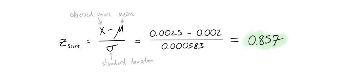
Then use a standard z-table to look up the probability associated with the above z-score.
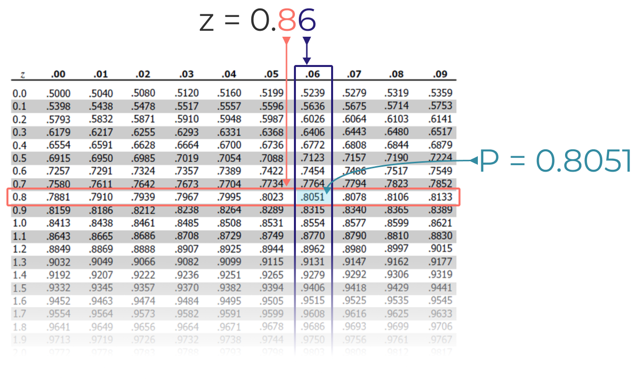
In this case we get a P value of 0.805, meaning 80.5% of all assemblies will be functional and 19.5% will require rework or be scrapped. That’s it!
Final Thoughts
The real world is messy and manufacturing issues are going to happen. The next time you and your team encounter a manufacturing or assembly issue you will now be armed with a powerful toolkit to understand and project costs and balance them against the cost of engineering and process improvements.
Five Flute - Next generation collaboration for hardware product development
If you are a design engineer or technical project manager and you want to design better products in less time, consider Five Flute. It’s the fastest way to share, review, and improve your engineering designs. From engineering drawing reviews to 3D design reviews of complex parts and assemblies, Five Flute is built for modern engineering teams that want to move faster without making mistakes.